Tree Analysis
Besides analysis based on table objects, BigObject solution also offers tree objects as the basis for analytics via tree analysis method. A tree object has a hierarchical structure that offers a more efficient way of computation than using a table object in some data analytics situations. BigObject provides a transformation mechanism called trans-join (transformative join) to construct a tree object from a table object. In general, there are three main procedures and one optional step involved in tree analysis. They are building the tree object, applying the function on the tree object, getting the data from the tree and store the result in a table.
The general syntax of creating a tree object is following:
CREATE TREE tree_name (data fields declaration on each node) FROM table_name GROUP BY each level specifiedColumns with data type VARSTRING or CHAR cannot be used in GROUP BY attributes when creating a tree.
In the example of ABC Company case, if the staff wants to create a tree object named T1 with two levels, Customer.gender and Product.brand. He can build such tree with following command:
CREATE TREE T1 (SUM(qty), tmp_d DOUBLE) FROM sales GROUP BY Customer.gender, Product.brandA tree T1 that looks like following in structure is created.
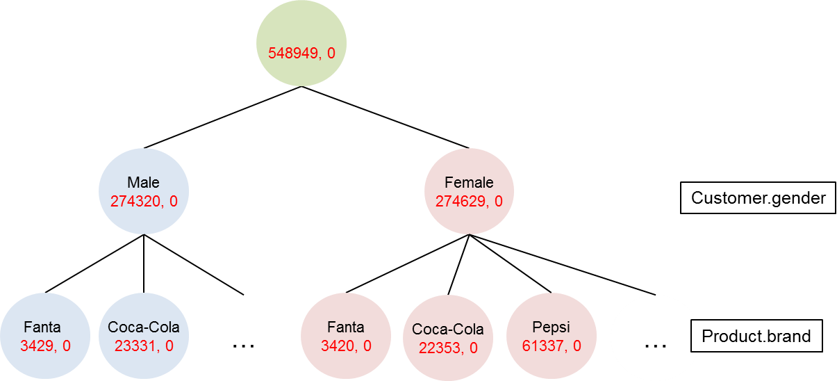
Each node in tree T1 holds two data fields, SUM(qty) and tmp_d. The value for SUM(qty) in each node is aggregated upward automatically through trans-join. The value of tmp_d is 0 for now, but it can be used to store the result of user-defined function.
Alternatively, the staff can also create a tree with same levels of declarations but contain more information and is more flexible for future use with CREATE ALL statement.
CREATE ALL TREE T2 (SUM(qty), tmp_d DOUBLE) FROM sales GROUP BY Customer.gender, Product.brandWith above command, a tree structure that looks like following is created.
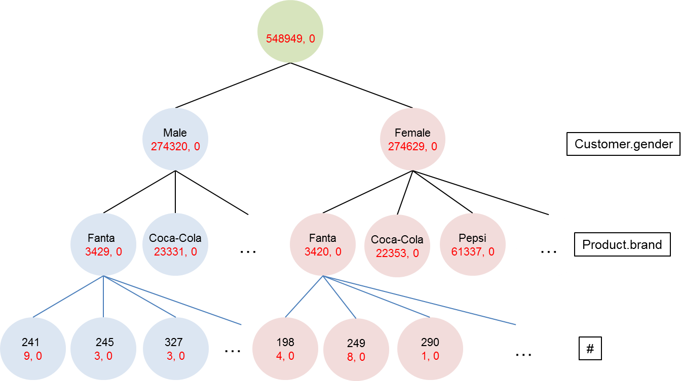
Build ALL will retain information for each transaction. The bottom level, commonly referred as "#", corresponds to each transaction in the sales table. It (Level #) contains the information of each transaction with its order ID (ID on each node) and transaction quantity (qty). Since the original qty data is preserved at leaf level #, it is possible to perform further analysis on TREE T2.
To query the data within the tree, a GET statement is required.
The general syntax for such GET statement is
GET data field FROM tree_name BY tree_pathA tree path can be a node name, asterisk(all nodes), index(-1 = last node) or a group of names seperated by '|':
| tree path | description |
|---|---|
| /Fanta | Level 1 'Fanta' node |
| /*/Iowa | Level 1 all nodes with Level 2 'Iowa' node |
| /Fanta/[-1] | Level 1 'Fanta node' and last node of Level 2 |
| /Powerade | Fanta/Iowa | Level 1'Powerade' and 'Fanta' nodes with Level 2 'Iowa' node |
For example, the following command returns toal quanties in Iowa for Fanta and Powerrade.
GET * FROM testtree1 BY '/Fanta|Powerade/Iowa'

+---------------+----------------+----+----------+
| Product.brand | Customer.state | v1 | SUM(qty) |
+---------------+----------------+----+----------+
| Fanta         | Iowa           |  0 |      138 |
| Powerade      | Iowa           |  0 |       46 |
+---------------+----------------+----+----------+
Finally, use CREATE TABLE statement to store the result in another table as follows:
CREATE TABLE table_name AS (GET statement for tree)Once the tree is built, the user can apply function on the tree object to do the analysis.
The general syntax for this is
APPLY function() TO tree_name AT specific level or tree pathLet's assume the staff of ABC company is interested to know which brand's 55% of quantity is coming from the top 20% of states (in quantity sold) using tree analysis.
The staff can first tran-join a tree from the sales table with the command:
CREATE TREE testtree1 (v1 DOUBLE, SUM(qty)) FROM sales GROUP BY Product.brand, Customer.stateThen apply pareto(55,20) function on the tree:
APPLY pareto(55,20) TO testtree1 AT Product.brand

+---------------+----------+----------+
| Product.brand | v1       | SUM(qty) |
+---------------+----------+----------+
| Coca-Cola     | 0.554639 |    46212 |
| Pepsi         | 0.557622 |   120840 |
| Mountain Dew  | 0.553333 |    10697 |
| Minute Maid   | 0.565028 |    17031 |
| Cheetos       | 0.556817 |    21763 |
| Propel        | 0.555525 |     7303 |
| Quaker Oats   | 0.580833 |     6198 |
| Dole          | 0.565848 |    31459 |
| Mirinda       | 0.569846 |     2076 |
| Ruffles       | 0.562246 |    20660 |
| Ocean Spray   | 0.571806 |    22317 |
| Lay's         | 0.567489 |    38325 |
| Doritos       | 0.556162 |    23468 |
| Quaker        |  0.55297 |    59770 |
| Sprite        | 0.552781 |     5447 |
| Powerade      | 0.555603 |     7095 |
| Aquarius      | 0.558772 |     2833 |
| Benenuts      | 0.552251 |    11464 |
| Looza         |  0.55605 |     1124 |
+---------------+----------+----------+
Those values that are greater than or equal to 0.55 under v1 column are the brands that have at least 55% of quantity sold from top 20 states.
Finally, ABC company staff can save the result into a table with following command:
CREATE TABLE saved_tree_result AS (APPLY pareto(55,20) TO testtree1 AT Product.brand)Auxiliary Clause:
The user can also place a filter condition in the GET statement.
Example:
GET v1, SUM(qty) FROM testtree1 BY '/*' WHERE v1 > 0.55The user can also arrange the order shown in the GET statement with sortby command.
Example:
GET v1, SUM(qty) FROM testtree1 BY '/*' order by v1